A Journey Full of Graphs

A little introduction

The implementation of the algorithm for NetworkX can be found here.

In discrete mathematics, a graph is a structure amounting to a set of objects in which some pairs of them are in some sense “related”. The objects are called vertices (also nodes) and each of the related pairs of vertices is called an edge. Fancy definition for just a simple representation that everyone probably has already seen one, but let’s give an example graph.

So as the circles seen at the above image are the so-called nodes and the edges are the lines that connect these circles.

The organization I worked for during the summer (and I plan on keep contributing afterwards) is NetworkX which is a Python package that implements data structures for graphs and has a lot of tools in order to explore these structures.

Now there are a lot of things we can say about graphs (it would take a lot of time and it isn’t part of this blog’s scope) but I will stick to my project.

Community Detection

The area of community detection focuses on grouping different nodes of a graph based on similar characteristics or the number of edges that connect them.

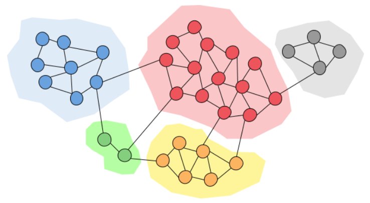
As we can see in the above image we can find some inner structure inside our graph, meaning that some nodes are more connected than others. We can basically group them together and say that these nodes belong to the same community. Grouping nodes of a network into communities has a lot of value since it can reveal a lot of information about the network itself. Communities can allow us to create a large scale map of a network since individual communities act like meta-nodes in the network which makes it easier to study. Also, communities often have very different properties than the average properties of the graph, giving us much more important information about the network etc.

So community detection is quite important. But you may wonder, how do we do it? We can’t really give a definitive answer to this question, because a community is an abstract idea. Also, the partition of a network into communities of densely connected nodes, with the nodes belonging to different communities being only sparsely connected is very hard computationally. In any case, there are a lot of algorithms that try to group nodes together based on some measures or the number of edges between nodes in reasonable timings.

Louvain Community Detection Algorithm

One of the algorithms I mentioned above is the Louvain method. It is a heuristic method (meaning that it isn’t perfect but produces quite good and often sufficient results) to extract the community structure of large networks. The method is based on modularity optimization and it is shown to be particularly fast and produces very good quality communities based on the modularity measure.

The modularity of a partition is a scalar value between -1 and 1 that measures the density of edges inside communities as compared to edges between communities. In the case of weighted networks (weighted networks are networks that have weights on their edges), it is defined as:

\[Q = \frac{1}{2m}\sum_{i,j}\left[A_{ij} - \frac{k_{i}k_{j}}{2m}\right]\delta(c_{i}, c_{j})\]

where \(A_{ij}\) represents the weight of the edge between \(i\) and \(j\), \(k_i=\sum_jA_{ij}\) is the sum of the weights of the edges attached to node \(i\), \(c_i\) is the community to which node \(i\) is assigned, the \(\delta\)-function \(\delta(u, v)\) is 1 if \(u=v\) and 0 otherwise and \(m=\frac{1}{2}\sum_{i,j}A_{ij}\).

The Louvain Method

Now that we have made some necessary definitions, let’s explore how the Louvain Community Detection algorithm works. The method consists of two phases. Assuming a weighted network of \(N\) nodes, we first assign a different community to each node. Then, for each node \(i\) we consider the neighbours \(j\) of \(i\) and we evaluate the gain of modularity that would take place by removing \(i\) from its community and by placing it in the community of \(j\). The node \(i\) is then placed in the community for which this gain is maximum, but only if the gain is positive. If no positive gain is possible, \(i\) stays in its original community. We repeat this process for all nodes until no further moves can occur. The latter sentence means that each node may be considered multiple times. The above process signifies the first phase. Let’s also note that the order with which we consider nodes do not seem to affect much the final modularity of the partition but can influence the computational time. The first phase is efficient because it is quite easy to compute the modularity gain \(\Delta Q\) by moving a node \(i\) into a community \(C\) from the following formula:

\[\Delta Q = \frac{k_{i,in}}{2m} - \gamma\frac{\Sigma_{tot} \cdot k_i}{2m^2}\]

where \(m\) is the size of the graph, \(k_{i,in}\) is the sum of the weights of the edges from \(i\) to nodes in \(C\), \(k_i\) is the sum of the weights of the edges incident to node \(i\), \(\Sigma_{tot}\) is the sum of the weights of the edges incident to nodes in \(C\) and \(\gamma\) is the resolution parameter (which can give a bias towards bigger communities if is is smaller than \(1\) and the smaller communities otherwise).

The second phase consists of building a new graph whose nodes are now the communities that we found during the first phase and the weights of the new edges between the new nodes are given by the sum of the weight of the edges between nodes in the corresponding communities. Links between nodes of the same community lead to self-loops. Once the new graph is created, it is possible to reapply the first phase.

We therefore, define a “pass” to be a combination of these two phases. The passes are iterated until there are no more changes and a local maximum of modularity it achieved. Consequently, the algorithm incorporates a notion of hierarchy, since a partition is created after each pass. An small example illustration of the method can be found in the following image where we see the grouping of nodes (first phase) and the creation of a new graph (second phase) and the second pass where the process repeats producing a smaller network at each step.

On first thought the algorithm can seem particularly slow given that we iterate all the nodes more than once, but the efficiency comes from the fact that the number of communities decreases drastically after just a few passes and so most of the computation takes place on the first iterations.

Just for completeness before I jump into the code presentation, I provide also the formula for modularity gain of a directed networkx in order to show that it is actual easy to make the algorithm compatible with directed graphs.

\[\Delta Q = \frac{k_{i,in}}{m} - \gamma\frac{k_i^{out} \cdot\Sigma_{tot}^{in} + k_i^{in} \cdot \Sigma_{tot}^{out}}{m^2}\]

where \(k_i^{out}\), \(k_i^{in}\) are the outer and inner weighted degrees of node \(i\) and \(\Sigma_{tot}^{in}\), \(\Sigma_{tot}^{out}\) are the sum of in-going and out-going edges incident to nodes in \(C\).

Implementing everything in Python

The implementation of the algorithm for NetworkX can be found here.

As described above, the algorithm produces a kind of hierarchy as we repeat each pass creating some kind of dendrogram. For that reason, we decided with my mentors to create 2 public functions, one is a generator (louvain_partitions) which yields a partition after every pass and one function (louvain_communities) which returns the last level of the tree which is the best partition in terms of modularity.

Both functions use the same loop which implements the passes.

m = graph.size(weight="weight")
partition, inner_partition, improvement = _one_level(
	graph, m, partition, resolution, is_directed, seed
)
improvement = True
while improvement:
    yield partition
    new_mod = modularity(
        graph, inner_partition, resolution=resolution, weight="weight"
    )
    if new_mod - mod <= threshold:
        return
    graph = _gen_graph(graph, inner_partition)
    partition, inner_partition, improvement = _one_level(
        graph, m, partition, resolution, is_directed, seed
    )

Just like the algorithm, the idea is simple. We compute the first level (using _one_level function which basically implements the first phase), we yield a partition every time there is an improvement (which means that there was at least one node moved from its community to another) and then we create a new graph from the partition we computed (using _gen_graph which implements the second phase). There is also the option to set a modularity gain threshold, meaning that the algorithm would stop if the gain achieved by one iteration isn’t bigger than a number specified by the user.

In order to get the bottom of the tree, ie the best partition, we just return the last partition yielded by the above loop which is what the louvain_communities function does.

Also, we chose to represent the partitions as a list of sets, each set containing the nodes that belong to the community. Ex. [{0,3,5,6}, {1,2,4}] is a partition of 2 communities, each containing the corresponding nodes.

The biggest challenge to implement was the _one_level function. Again the idea of the algorithm is simple: Randomly iterate through all the nodes and for every one of their neighbours check the modularity gain obtained by moving the specific node to the neighbor community and finally move it to the group which has the maximum positive gain, otherwise it stays where it is.

But, since there are a lot of nested loops the timing for the algorithm wasn’t very good (nowhere near on the numbers they presented on the original paper) and the reason for that is that Python is much slower than C++. I had to use a lot of data structures to precompute some of the factors of the modularity gain formula which would speed up things by removing inner loops.

Additionally, I created a helper function _neighbor_weights which takes a dictionary of a node’s neighbours and their respected weights as input and computes the total weight of the node to every one of its neighbour communities. This function basically calculates the \(k_{i,in}\) parameter from the modularity gain formula.

Let us note that the order in which the nodes are chosen is random using the shuffle function.

So after a lot of trial and errors the _one_level function was working and was quite fast (dare to say a little faster than this Python implementation for Louvain algorithm).

Next was the second phase (ie generate a new graph based on the communities computed on the first phase) which is implemented by the _gen_graph function. Again it is a simple idea, first I add the nodes to a new graph that represent and hold the communities, and then I sum the weights of the edges between the old nodes that constitute the communities in order to calculate the new edges between the new nodes in the meta-graph.

Conclusion

I hope I managed to give a good idea of the work I did during the summer and to explain how the Louvain Community Detection method works. Overall it was a great learning experience on which I learned a lot of stuff and had a lot of fun coding. I would like to thank my mentors Dan Schult and Mridul Seth for their help, guidance and friendship. Also every one of the core developers of NetworkX was very friendly and willing to help making me fill very comfortable during my entire work period. I will definitely stay in touch and keep contributing to this great community.